Multi-slide analysis and score transfer (Colon Day 9)
2026-05-10
Source:vignettes/colon_d9_multi_slide.Rmd
colon_d9_multi_slide.RmdOverview
This vignette demonstrates CoPro’s multi-slide analysis and score transfer capabilities using colon organoid Day 9 data. At Day 9, the tissue exhibits severe inflammation with heterogeneous disease progression across different regions. CoPro detects a disease progression axis that correlates with independently derived mucosal neighborhood (MU) labels—in particular, MU8 marks the most severely inflamed niche.
When multiple tissue slides are available, CoPro can:
- Learn co-progression patterns from a reference slide
- Transfer the learned gene weights to new slides
- Compare co-progression patterns across biological replicates
Download and load data
data_path <- copro_download_data("colon_d9")## Downloading copro_colon_d9.rds from GitHub Release 'data-v1'...## Downloaded to: /home/runner/.cache/R/CoPro/copro_colon_d9.rds
dat <- readRDS(data_path)

# Three slides are included
cat("Slides:", paste(dat$selectedSlides, collapse = ", "), "\n")
## Slides: 062221_D9_m3_2_slice_1, 062221_D9_m3_2_slice_2, 062221_D9_m3_2_slice_3## Total cells: 21436
table(dat$slideID)##
## 062221_D9_m3_2_slice_1 062221_D9_m3_2_slice_2 062221_D9_m3_2_slice_3
## 7242 6627 7567Visualize the tissue
Cell types
plot_df <- data.frame(
  x = dat$locationData$x,
  y = dat$locationData$y,
  celltype = dat$cellTypes,
  slide = dat$slideID
)

ggplot(plot_df[plot_df$slide == dat$selectedSlides[1], ],
       aes(x = x, y = y, color = celltype)) +
  geom_point(size = 0.5, alpha = 0.6) +
  scale_color_manual(values = c("Epithelial" = "#E41A1C",
                                 "Fibroblast" = "#377EB8",
                                 "Immune" = "#4DAF4A")) +
  coord_fixed() +
  ggtitle(paste("Colon Day 9 --", dat$selectedSlides[1])) +
  theme_classic() +
  theme(legend.position = "bottom")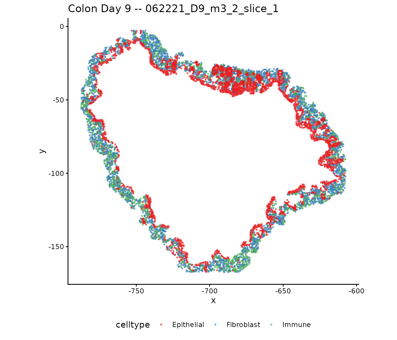
Mucosal neighborhood (MU) labels
The tissue has been independently annotated with mucosal neighborhood labels via Leiden clustering. MU8 marks the most severely inflamed niche, while MU1–3 are grouped as relatively normal crypt neighborhoods:
mu_df <- data.frame(
  x = dat$locationData$x,
  y = dat$locationData$y,
  MU = dat$metaData$Leiden_neigh,
  slide = dat$slideID
)

# Group MU labels as in the manuscript
mu_df$MU_grouped <- as.character(mu_df$MU)
mu_df$MU_grouped[mu_df$MU %in% c("MU1", "MU11")] <- "MU1-3"
mu_df <- mu_df[mu_df$MU_grouped %in% c("MU1-3", "MU5", "MU6", "MU7", "MU8"), ]
mu_df$MU_grouped <- factor(mu_df$MU_grouped,
                            levels = c("MU1-3", "MU5", "MU6", "MU7", "MU8"))

mu_colors <- c("MU1-3" = "#66C2A5", "MU5" = "#E5C494",
               "MU6" = "#8DA0CB", "MU7" = "#FC8D62", "MU8" = "#E78AC3")

ggplot(mu_df[mu_df$slide == dat$selectedSlides[1], ],
       aes(x = x, y = y, color = MU_grouped)) +
  geom_point(size = 0.5) +
  scale_color_manual(values = mu_colors) +
  coord_fixed() +
  ggtitle("Mucosal neighborhoods (MU labels)") +
  theme_classic() +
  theme(legend.title = element_blank(), legend.position = "right") +
  guides(color = guide_legend(override.aes = list(size = 3)))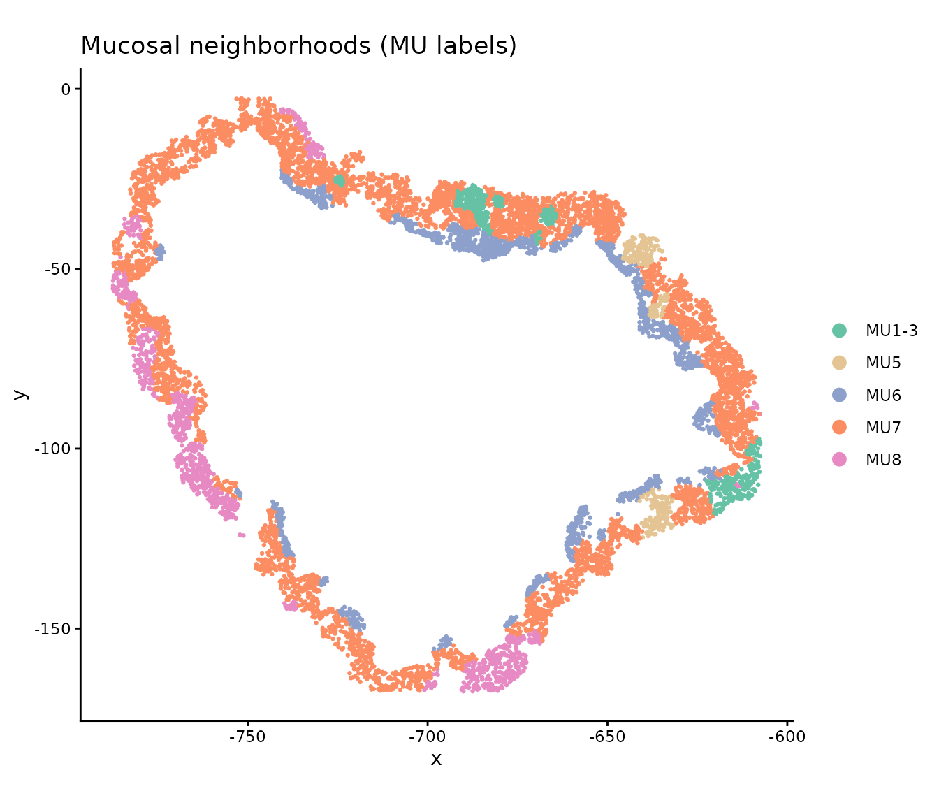
Strategy: Reference + target slides
We use the first slide as the reference to learn co-progression patterns, then transfer scores to the other two slides.
ref_slide <- dat$selectedSlides[1]
tar_slides <- dat$selectedSlides[2:3]

# Indices for reference and target
ref_idx <- dat$slideID == ref_slide
tar1_idx <- dat$slideID == tar_slides[1]
tar2_idx <- dat$slideID == tar_slides[2]
Step 1: Run CoPro on the reference slide
cell_types <- c("Epithelial", "Fibroblast", "Immune")

# Create reference CoPro object
ref_obj <- newCoProSingle(
  normalizedData = dat$normalizedData[ref_idx, ],
  locationData = dat$locationData[ref_idx, ],
  metaData = dat$metaData[ref_idx, ],
  cellTypes = dat$cellTypes[ref_idx]
)
ref_obj <- subsetData(ref_obj, cellTypesOfInterest = cell_types)

# Run pipeline
ref_obj <- computePCA(ref_obj, nPCA = 40, center = TRUE, scale. = TRUE)
## Input is dense (matrixarray), performing irlba pca...
## Input is dense (matrixarray), performing irlba pca...
## Input is dense (matrixarray), performing irlba pca...
ref_obj <- computeDistance(ref_obj, distType = "Euclidean2D")## normalizeDistance = TRUE: low-percentile distance will be scaled to 0.01.## 0% 25% 50% 75% 100%
## 1.559086 54.812663 95.648432 126.009495 191.917943
## 0% 25% 50% 75% 100%
## 1.723399 61.128716 100.304344 127.403172 191.878277
## 0% 25% 50% 75% 100%
## 1.033183 59.470179 102.405454 133.908593 194.179085## Distance normalization scaling factor: 0.00967883
sigma_choice <- c(0.005, 0.01, 0.02, 0.05, 0.1)
ref_obj <- computeKernelMatrix(ref_obj, sigmaValues = sigma_choice)
## Computing pairwise kernel matrix for 3 cell types
## current sigma value is 0.005
## current sigma value is 0.01
## current sigma value is 0.02
## current sigma value is 0.05
## current sigma value is 0.1
ref_obj <- runSkrCCA(ref_obj, scalePCs = TRUE, maxIter = 500, nCC = 2)## Running skrCCA [1/5] for sigma = 0.005 ...## [1] "Convergence reached at 10 iterations (Max diff = 8.855e-06 )"
## [1] "Convergence reached at 40 iterations (Max diff = 8.130e-06 )"## Running skrCCA [2/5] for sigma = 0.01 ...## [1] "Convergence reached at 10 iterations (Max diff = 7.128e-06 )"
## [1] "Convergence reached at 9 iterations (Max diff = 3.697e-06 )"## Running skrCCA [3/5] for sigma = 0.02 ...## [1] "Convergence reached at 9 iterations (Max diff = 6.981e-06 )"
## [1] "Convergence reached at 8 iterations (Max diff = 5.635e-06 )"## Running skrCCA [4/5] for sigma = 0.05 ...## [1] "Convergence reached at 8 iterations (Max diff = 4.572e-06 )"
## [1] "Convergence reached at 9 iterations (Max diff = 2.760e-06 )"## Running skrCCA [5/5] for sigma = 0.1 ...## [1] "Convergence reached at 6 iterations (Max diff = 5.352e-06 )"
## [1] "Convergence reached at 7 iterations (Max diff = 2.794e-06 )"## skrCCA finished 5 sigma value(s) in 5.7 s.## Optimization succeeded for 5 sigma value(s): sigma_0.005, sigma_0.01, sigma_0.02, sigma_0.05, sigma_0.1
ref_obj <- computeNormalizedCorrelation(ref_obj)## Calculating spectral norms, this may take a while.## Finished calculating spectral norms.
ref_obj <- computeGeneAndCellScores(ref_obj)
ref_obj <- computeRegressionGeneScores(ref_obj)
## Computed regression gene scores for sigma=0.005, cellType='Epithelial'## Computed regression gene scores for sigma=0.005, cellType='Fibroblast'## Computed regression gene scores for sigma=0.005, cellType='Immune'## Computed regression gene scores for sigma=0.01, cellType='Epithelial'## Computed regression gene scores for sigma=0.01, cellType='Fibroblast'## Computed regression gene scores for sigma=0.01, cellType='Immune'## Computed regression gene scores for sigma=0.02, cellType='Epithelial'## Computed regression gene scores for sigma=0.02, cellType='Fibroblast'## Computed regression gene scores for sigma=0.02, cellType='Immune'## Computed regression gene scores for sigma=0.05, cellType='Epithelial'## Computed regression gene scores for sigma=0.05, cellType='Fibroblast'## Computed regression gene scores for sigma=0.05, cellType='Immune'## Computed regression gene scores for sigma=0.1, cellType='Epithelial'## Computed regression gene scores for sigma=0.1, cellType='Fibroblast'## Computed regression gene scores for sigma=0.1, cellType='Immune'Reference slide results
sigma_opt <- 0.01  # adjust based on normalized correlation

cs_ref <- getCellScoresInSitu(ref_obj, sigmaValueChoice = sigma_opt)

ggplot(cs_ref) +
  geom_point(aes(x = x, y = y, color = cellScores), size = 0.8) +
  scale_color_viridis_c() +
  facet_wrap(~ cellTypesSub) +
  coord_fixed() +
  ggtitle(paste("Reference slide:", ref_slide)) +
  theme_minimal()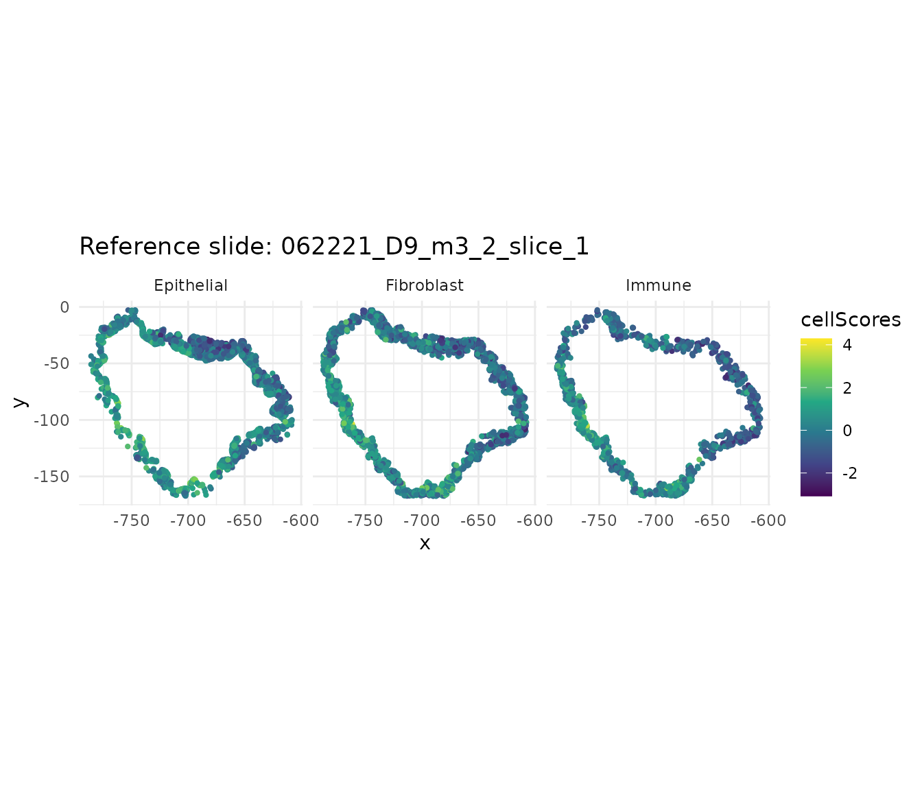
Disease axis vs MU labels
The CoPro disease axis should correlate with MU labels, with MU8 cells showing the highest scores:
ref_meta <- ref_obj@metaDataSub
ref_meta$cell_score <- ref_meta[, paste0("cellScore_sigma_", sigma_opt,
                                          "_cc_index_1")]

# Assign grouped MU labels
ref_meta$MU_grouped <- as.character(ref_meta$Leiden_neigh)
ref_meta$MU_grouped[ref_meta$MU_grouped %in% c("MU1", "MU11")] <- "MU1-3"
ref_meta <- ref_meta[ref_meta$MU_grouped %in%
                      c("MU1-3", "MU5", "MU6", "MU7", "MU8"), ]
ref_meta$MU_grouped <- factor(ref_meta$MU_grouped,
                               levels = c("MU1-3", "MU5", "MU6", "MU7", "MU8"))

ggplot(ref_meta, aes(x = MU_grouped, y = cell_score, fill = MU_grouped)) +
  geom_boxplot(outlier.size = 0.3) +
  scale_fill_manual(values = mu_colors, guide = "none") +
  labs(x = "Mucosal Neighborhood", y = "CoPro disease score (CC1)",
       title = "Disease scores by MU label",
       subtitle = "MU8 = most inflamed niche") +
  theme_classic()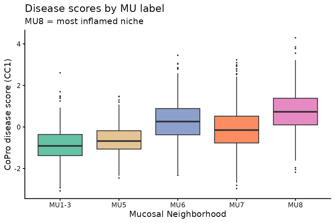
Cell type proportions along the disease axis
As disease severity increases, the cell type composition shifts—immune cell proportion increases while epithelial proportion decreases:
ref_meta_all <- ref_obj@metaDataSub
ref_meta_all$cell_score <- ref_meta_all[, paste0("cellScore_sigma_",
                                                   sigma_opt, "_cc_index_1")]

# Bin cells by disease score
ref_meta_all$score_bin <- cut(ref_meta_all$cell_score, breaks = 20)

# Calculate proportions
prop_df <- do.call(rbind, lapply(split(ref_meta_all, ref_meta_all$score_bin),
  function(x) {
    data.frame(
      score_mid = mean(x$cell_score, na.rm = TRUE),
      Epithelial = mean(x$Tier1 == "Epithelial"),
      Fibroblast = mean(x$Tier1 == "Fibroblast"),
      Immune = mean(x$Tier1 == "Immune")
    )
  }
))
prop_long <- reshape(prop_df, direction = "long",
                     varying = c("Epithelial", "Fibroblast", "Immune"),
                     v.names = "proportion", timevar = "celltype",
                     times = c("Epithelial", "Fibroblast", "Immune"))

ggplot(prop_long, aes(x = score_mid, y = proportion, color = celltype)) +
  geom_point() +
  geom_smooth(method = "loess", se = FALSE) +
  scale_color_manual(values = c("Epithelial" = "#E41A1C",
                                 "Fibroblast" = "#377EB8",
                                 "Immune" = "#4DAF4A")) +
  labs(x = "CoPro disease score (CC1)", y = "Cell type proportion",
       title = "Cell type composition along the disease axis") +
  theme_classic() +
  theme(legend.position = "bottom")
## `geom_smooth()` using formula = 'y ~ x'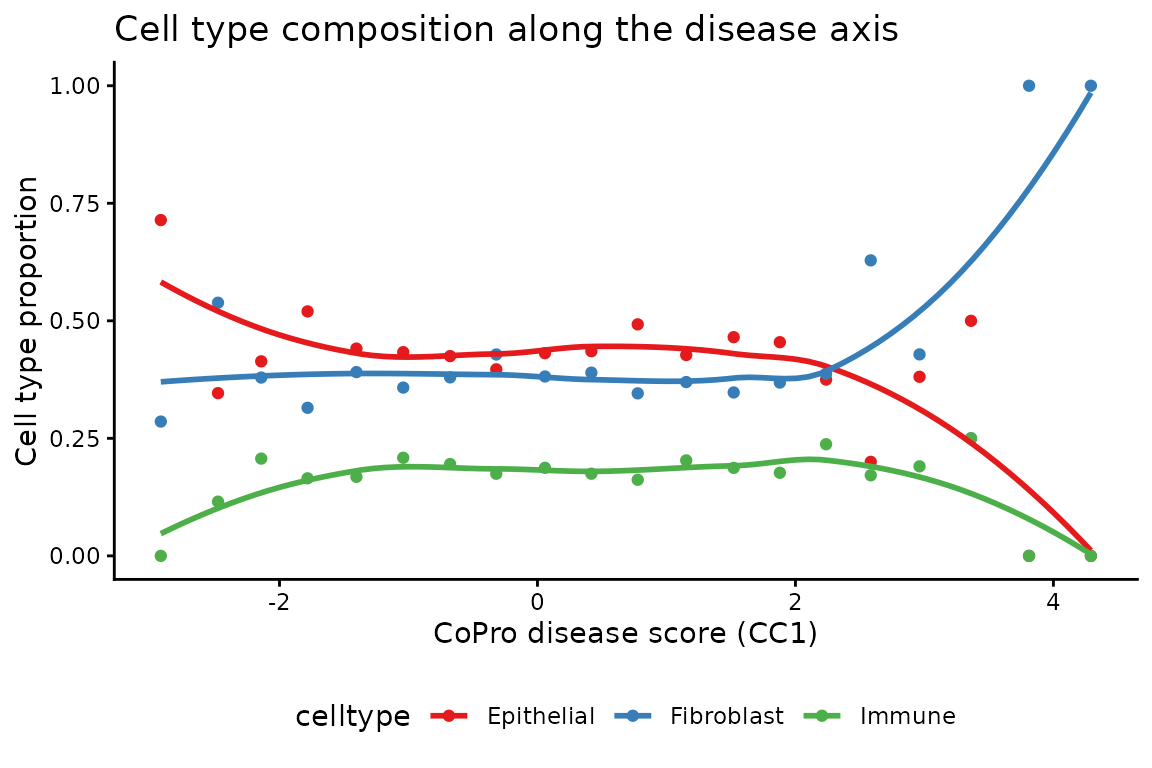
Top genes associated with the disease axis
# Immune genes on the disease axis
key_imm <- paste0("geneScores|sigma", sigma_opt, "|Immune")
gs_imm <- ref_obj@geneScoresRegression[[key_imm]]
gs_imm_cc1 <- gs_imm[, 1]

top_imm <- head(sort(abs(gs_imm_cc1), decreasing = TRUE), 20)
top_imm_df <- data.frame(
  gene = factor(names(top_imm), levels = rev(names(top_imm))),
  weight = gs_imm_cc1[names(top_imm)]
)
top_imm_df$direction <- ifelse(top_imm_df$weight > 0, "inflamed", "normal")

ggplot(top_imm_df, aes(x = gene, y = weight, fill = direction)) +
  geom_col() +
  coord_flip() +
  scale_fill_manual(values = c("inflamed" = "darkgreen",
                                "normal" = "lightgreen")) +
  ggtitle("Top 20 Immune genes (CC1, regression)") +
  theme_classic() +
  theme(legend.position = "bottom")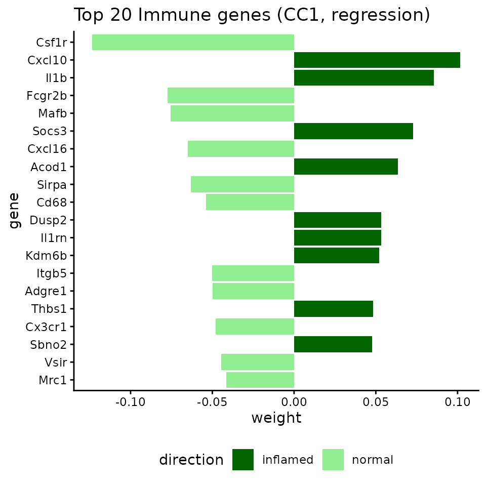
Step 2: Create target CoPro objects
# Target slide 1
tar1_obj <- newCoProSingle(
  normalizedData = dat$normalizedData[tar1_idx, ],
  locationData = dat$locationData[tar1_idx, ],
  metaData = dat$metaData[tar1_idx, ],
  cellTypes = dat$cellTypes[tar1_idx]
)
tar1_obj <- subsetData(tar1_obj, cellTypesOfInterest = cell_types)
tar1_obj <- computePCA(tar1_obj, nPCA = 40, center = TRUE, scale. = TRUE)
## Input is dense (matrixarray), performing irlba pca...
## Input is dense (matrixarray), performing irlba pca...
## Input is dense (matrixarray), performing irlba pca...
tar1_obj <- computeDistance(tar1_obj, distType = "Euclidean2D")## normalizeDistance = TRUE: low-percentile distance will be scaled to 0.01.## 0% 25% 50% 75% 100%
## 1.547908 40.150567 71.639135 99.196604 145.064234
## 0% 25% 50% 75% 100%
## 1.839067 46.588659 74.794733 100.618483 144.602279
## 0% 25% 50% 75% 100%
## 1.077755 44.939240 73.568954 97.010170 146.985239## Distance normalization scaling factor: 0.00927854
tar1_obj <- computeKernelMatrix(tar1_obj, sigmaValues = sigma_choice)## Computing pairwise kernel matrix for 3 cell types
## current sigma value is 0.005
## current sigma value is 0.01
## current sigma value is 0.02
## current sigma value is 0.05
## current sigma value is 0.1
# Target slide 2
tar2_obj <- newCoProSingle(
  normalizedData = dat$normalizedData[tar2_idx, ],
  locationData = dat$locationData[tar2_idx, ],
  metaData = dat$metaData[tar2_idx, ],
  cellTypes = dat$cellTypes[tar2_idx]
)
tar2_obj <- subsetData(tar2_obj, cellTypesOfInterest = cell_types)
tar2_obj <- computePCA(tar2_obj, nPCA = 40, center = TRUE, scale. = TRUE)
## Input is dense (matrixarray), performing irlba pca...
## Input is dense (matrixarray), performing irlba pca...
## Input is dense (matrixarray), performing irlba pca...
tar2_obj <- computeDistance(tar2_obj, distType = "Euclidean2D")## normalizeDistance = TRUE: low-percentile distance will be scaled to 0.01.## 0% 25% 50% 75% 100%
## 1.65134 41.19449 71.21469 94.13571 147.60112
## 0% 25% 50% 75% 100%
## 2.021933 50.297768 74.971212 97.972906 148.666374
## 0% 25% 50% 75% 100%
## 1.162089 43.393514 70.036161 92.718582 149.327113## Distance normalization scaling factor: 0.0086052
tar2_obj <- computeKernelMatrix(tar2_obj, sigmaValues = sigma_choice)## Computing pairwise kernel matrix for 3 cell types
## current sigma value is 0.005
## current sigma value is 0.01
## current sigma value is 0.02
## current sigma value is 0.05
## current sigma value is 0.1Step 3: Transfer scores
Transfer the learned gene weights from the reference to each target slide:
# Transfer to target 1
tar1_scores <- getTransferCellScores(
  ref_obj = ref_obj,
  tar_obj = tar1_obj,
  sigma_choice = sigma_opt,
  gene_score_type = "regression"
)
## Using regression-based gene weights for transfer
## transferring gene scores for cell type Epithelial## Processing feature 94/940## Processing feature 188/940## Processing feature 282/940## Processing feature 376/940## Processing feature 470/940## Processing feature 564/940## Processing feature 658/940## Processing feature 752/940## Processing feature 846/940## Processing feature 940/940## retaining 940 genes for CC_1 with threshold 0
## retaining 940 genes for CC_2 with threshold 0
## transferring gene scores for cell type Fibroblast## Processing feature 94/940## Processing feature 188/940## Processing feature 282/940## Processing feature 376/940## Processing feature 470/940## Processing feature 564/940## Processing feature 658/940## Processing feature 752/940## Processing feature 846/940## Processing feature 940/940## retaining 940 genes for CC_1 with threshold 0
## retaining 940 genes for CC_2 with threshold 0
## transferring gene scores for cell type Immune## Processing feature 94/940## Processing feature 188/940## Processing feature 282/940## Processing feature 376/940## Processing feature 470/940## Processing feature 564/940## Processing feature 658/940## Processing feature 752/940## Processing feature 846/940## Processing feature 940/940## retaining 940 genes for CC_1 with threshold 0
## retaining 940 genes for CC_2 with threshold 0
# Transfer to target 2
tar2_scores <- getTransferCellScores(
  ref_obj = ref_obj,
  tar_obj = tar2_obj,
  sigma_choice = sigma_opt,
  gene_score_type = "regression"
)
## Using regression-based gene weights for transfer
## transferring gene scores for cell type Epithelial## Processing feature 94/940## Processing feature 188/940## Processing feature 282/940## Processing feature 376/940## Processing feature 470/940## Processing feature 564/940## Processing feature 658/940## Processing feature 752/940## Processing feature 846/940## Processing feature 940/940## retaining 940 genes for CC_1 with threshold 0
## retaining 940 genes for CC_2 with threshold 0
## transferring gene scores for cell type Fibroblast## Processing feature 94/940## Processing feature 188/940## Processing feature 282/940## Processing feature 376/940## Processing feature 470/940## Processing feature 564/940## Processing feature 658/940## Processing feature 752/940## Processing feature 846/940## Processing feature 940/940## retaining 940 genes for CC_1 with threshold 0
## retaining 940 genes for CC_2 with threshold 0
## transferring gene scores for cell type Immune## Processing feature 94/940## Processing feature 188/940## Processing feature 282/940## Processing feature 376/940## Processing feature 470/940## Processing feature 564/940## Processing feature 658/940## Processing feature 752/940## Processing feature 846/940## Processing feature 940/940## retaining 940 genes for CC_1 with threshold 0
## retaining 940 genes for CC_2 with threshold 0Step 4: Visualize transferred scores
# Build data frames for target slides from transferred scores
build_transfer_df <- function(tar_dat, tar_scores, slide_name, sigma) {
  rows <- list()
  for (ct in cell_types) {
    ct_key <- paste0("geneScores|sigma", sigma, "|", ct)
    if (ct_key %in% names(tar_scores)) {
      ct_idx <- tar_dat$cellTypes == ct
      rows[[ct]] <- data.frame(
        x = tar_dat$locationData$x[ct_idx],
        y = tar_dat$locationData$y[ct_idx],
        cellScores = tar_scores[[ct_key]][, 1],
        cellTypesSub = ct,
        slide = slide_name
      )
    }
  }
  do.call(rbind, rows)
}

# Build target data using the original dat split by slide indices
tar1_dat <- list(
  locationData = dat$locationData[tar1_idx, ],
  cellTypes = dat$cellTypes[tar1_idx]
)
tar2_dat <- list(
  locationData = dat$locationData[tar2_idx, ],
  cellTypes = dat$cellTypes[tar2_idx]
)

tar1_cs <- build_transfer_df(tar1_dat, tar1_scores, tar_slides[1], sigma_opt)
tar2_cs <- build_transfer_df(tar2_dat, tar2_scores, tar_slides[2], sigma_opt)

# Add slide label to reference
cs_ref$slide <- ref_slide

all_cs <- rbind(
  cs_ref[, c("x", "y", "cellScores", "cellTypesSub", "slide")],
  tar1_cs,
  tar2_cs
)

ggplot(all_cs) +
  geom_point(aes(x = x, y = y, color = cellScores), size = 0.5) +
  scale_color_viridis_c() +
  facet_grid(slide ~ cellTypesSub) +
  coord_fixed() +
  ggtitle("CC1 scores: reference (top) vs transferred (bottom)") +
  theme_minimal() +
theme(strip.text = element_text(size = 8))![]()
Step 5: Transferred scores vs MU labels on target slides
Check whether the transferred disease scores also separate MU labels. Here we show the reference slide MU boxplot (already computed above) alongside the MU labels in spatial context for a target slide:
# Show MU labels spatially on target slide 1
tar1_mu <- data.frame(
  x = dat$locationData$x[tar1_idx],
  y = dat$locationData$y[tar1_idx],
  MU = dat$metaData$Leiden_neigh[tar1_idx]
)
tar1_mu$MU_grouped <- as.character(tar1_mu$MU)
tar1_mu$MU_grouped[tar1_mu$MU_grouped %in% c("MU1", "MU11")] <- "MU1-3"
tar1_mu <- tar1_mu[tar1_mu$MU_grouped %in%
                    c("MU1-3", "MU5", "MU6", "MU7", "MU8"), ]
tar1_mu$MU_grouped <- factor(tar1_mu$MU_grouped,
                              levels = c("MU1-3", "MU5", "MU6", "MU7", "MU8"))

ggplot(tar1_mu, aes(x = x, y = y, color = MU_grouped)) +
  geom_point(size = 0.5) +
  scale_color_manual(values = mu_colors) +
  coord_fixed() +
  ggtitle(paste("MU labels --", tar_slides[1])) +
  theme_classic() +
theme(legend.title = element_blank())![]()
Step 6: Assess transfer consistency
Compare the normalized correlation between the reference and transferred slides to assess whether the co-progression pattern is consistent:
tar1_ncorr <- getTransferNormCorr(
  tar_obj = tar1_obj,
  transfer_cell_scores = tar1_scores,
  sigma_choice = sigma_opt
)
## Calculating spectral norms, this may take a while.## Finished calculating spectral norms.
tar2_ncorr <- getTransferNormCorr(
  tar_obj = tar2_obj,
  transfer_cell_scores = tar2_scores,
  sigma_choice = sigma_opt
)
## Calculating spectral norms, this may take a while.
## Finished calculating spectral norms.
cat("Reference norm. corr.:\n")## Reference norm. corr.:
ref_ncorr <- getNormCorr(ref_obj)
print(ref_ncorr[ref_ncorr$sigmaValues == sigma_opt, ])
## sigmaValues cellType1 cellType2 CC_index normalizedCorrelation
## sigma_0.01.1 0.01 Epithelial Fibroblast 1 0.1347933
## sigma_0.01.2 0.01 Epithelial Immune 1 0.1172362
## sigma_0.01.3 0.01 Fibroblast Immune 1 0.2806241
## sigma_0.01.4 0.01 Epithelial Fibroblast 2 0.1584864
## sigma_0.01.5 0.01 Epithelial Immune 2 -0.0046844
## sigma_0.01.6 0.01 Fibroblast Immune 2 0.1101345
## ct12
## sigma_0.01.1 Epithelial-Fibroblast
## sigma_0.01.2 Epithelial-Immune
## sigma_0.01.3 Fibroblast-Immune
## sigma_0.01.4 Epithelial-Fibroblast
## sigma_0.01.5 Epithelial-Immune
## sigma_0.01.6 Fibroblast-Immune
cat("\nTarget 1 transferred norm. corr.:\n")##
## Target 1 transferred norm. corr.:
print(tar1_ncorr)## $sigma_0.01
## sigmaValue cellType1 cellType2 CC_index normalizedCorrelation
## 1 0.01 Epithelial Fibroblast 1 0.11110711
## 2 0.01 Epithelial Fibroblast 2 0.07360585
## 3 0.01 Epithelial Immune 1 0.10573678
## 4 0.01 Epithelial Immune 2 -0.07005265
## 5 0.01 Fibroblast Immune 1 0.29851289
## 6 0.01 Fibroblast Immune 2 0.10033653
cat("\nTarget 2 transferred norm. corr.:\n")##
## Target 2 transferred norm. corr.:
print(tar2_ncorr)## $sigma_0.01
## sigmaValue cellType1 cellType2 CC_index normalizedCorrelation
## 1 0.01 Epithelial Fibroblast 1 0.06226175
## 2 0.01 Epithelial Fibroblast 2 0.08658253
## 3 0.01 Epithelial Immune 1 0.07693582
## 4 0.01 Epithelial Immune 2 -0.02331899
## 5 0.01 Fibroblast Immune 1 0.26800977
## 6 0.01 Fibroblast Immune 2 0.09241650High transferred normalized correlations indicate that the co-progression pattern learned from the reference generalizes well to independent slides.
Alternative: Multi-slide CoPro
For joint analysis across all slides simultaneously, use
newCoProMulti:
multi_obj <- newCoProMulti(
  normalizedData = dat$normalizedData,
  locationData = dat$locationData,
  metaData = dat$metaData,
  cellTypes = dat$cellTypes,
  slideID = dat$slideID
)
multi_obj <- subsetData(multi_obj, cellTypesOfInterest = cell_types)

# The rest of the pipeline is identical
multi_obj <- computePCA(multi_obj, nPCA = 40, center = TRUE, scale. = TRUE)
## Performing PCA for cell type: Epithelial## Data centered and/or scaled## PCA computed for cell type: Epithelial## Performing PCA for cell type: Fibroblast## Data centered and/or scaled## PCA computed for cell type: Fibroblast## Performing PCA for cell type: Immune## Data centered and/or scaled## PCA computed for cell type: Immune
multi_obj <- computeDistance(multi_obj, distType = "Euclidean2D")## normalizeDistance = TRUE: low-percentile distance will be normalized across all slides and scaled to 0.01.## Computing pairwise distances for slide: 062221_D9_m3_2_slice_3## Slide: 062221_D9_m3_2_slice_3, Pair: Epithelial - Fibroblast## 0% 25% 50% 75% 100%
## 1.65134 41.19449 71.21469 94.13571 147.60112## Slide: 062221_D9_m3_2_slice_3, Pair: Epithelial - Immune## 0% 25% 50% 75% 100%
## 2.021933 50.297768 74.971212 97.972906 148.666374## Slide: 062221_D9_m3_2_slice_3, Pair: Fibroblast - Immune## 0% 25% 50% 75% 100%
## 1.162089 43.393514 70.036161 92.718582 149.327113## Computing pairwise distances for slide: 062221_D9_m3_2_slice_2## Slide: 062221_D9_m3_2_slice_2, Pair: Epithelial - Fibroblast## 0% 25% 50% 75% 100%
## 1.547908 40.150567 71.639135 99.196604 145.064234## Slide: 062221_D9_m3_2_slice_2, Pair: Epithelial - Immune## 0% 25% 50% 75% 100%
## 1.839067 46.588659 74.794733 100.618483 144.602279## Slide: 062221_D9_m3_2_slice_2, Pair: Fibroblast - Immune## 0% 25% 50% 75% 100%
## 1.077755 44.939240 73.568954 97.010170 146.985239## Computing pairwise distances for slide: 062221_D9_m3_2_slice_1## Slide: 062221_D9_m3_2_slice_1, Pair: Epithelial - Fibroblast## 0% 25% 50% 75% 100%
## 1.559086 54.812663 95.648432 126.009495 191.917943## Slide: 062221_D9_m3_2_slice_1, Pair: Epithelial - Immune## 0% 25% 50% 75% 100%
## 1.723399 61.128716 100.304344 127.403172 191.878277## Slide: 062221_D9_m3_2_slice_1, Pair: Fibroblast - Immune## 0% 25% 50% 75% 100%
## 1.033183 59.470179 102.405454 133.908593 194.179085## Global distance scaling factor: 0.00967883
multi_obj <- computeKernelMatrix(multi_obj, sigmaValues = sigma_choice)## Computing pairwise kernel matrix for 3 cell types across 3 slides
## current sigma value is 0.005
## current sigma value is 0.01
## current sigma value is 0.02
## current sigma value is 0.05
## current sigma value is 0.1
multi_obj <- runSkrCCA(multi_obj, scalePCs = TRUE, maxIter = 500, nCC = 2)## Running skrCCA [1/5] for sigma = 0.005 ...## Convergence reached at 8 iterations (Max diff = 6.856e-06 )## [1] "Convergence reached at 19 iterations (Max diff = 8.112e-06 )"## Running skrCCA [2/5] for sigma = 0.01 ...## Convergence reached at 8 iterations (Max diff = 2.045e-06 )## [1] "Convergence reached at 74 iterations (Max diff = 9.409e-06 )"## Running skrCCA [3/5] for sigma = 0.02 ...## Convergence reached at 7 iterations (Max diff = 4.600e-06 )## [1] "Convergence reached at 33 iterations (Max diff = 7.607e-06 )"## Running skrCCA [4/5] for sigma = 0.05 ...## Convergence reached at 7 iterations (Max diff = 7.622e-06 )## [1] "Convergence reached at 18 iterations (Max diff = 8.816e-06 )"## Running skrCCA [5/5] for sigma = 0.1 ...## Convergence reached at 10 iterations (Max diff = 1.994e-06 )## [1] "Convergence reached at 20 iterations (Max diff = 8.645e-06 )"## skrCCA finished 5 sigma value(s) in 14.3 s.## Optimization succeeded for 5 sigma value(s): sigma_0.005, sigma_0.01, sigma_0.02, sigma_0.05, sigma_0.1
multi_obj <- computeNormalizedCorrelation(multi_obj)## Calculating spectral norms (can take time)...## Finished calculating spectral norms.
multi_obj <- computeGeneAndCellScores(multi_obj)The multi-slide approach optimizes CCA weights jointly across all slides, while the transfer approach trains on one slide and evaluates generalization. Both are useful depending on your analytical question.
Session info
## R version 4.6.0 (2026-04-24)
## Platform: x86_64-pc-linux-gnu
## Running under: Ubuntu 24.04.4 LTS
##
## Matrix products: default
## BLAS:   /usr/lib/x86_64-linux-gnu/openblas-pthread/libblas.so.3
## LAPACK: /usr/lib/x86_64-linux-gnu/openblas-pthread/libopenblasp-r0.3.26.so;  LAPACK version 3.12.0
##
## locale:
##  [1] LC_CTYPE=C.UTF-8       LC_NUMERIC=C           LC_TIME=C.UTF-8
##  [4] LC_COLLATE=C.UTF-8     LC_MONETARY=C.UTF-8    LC_MESSAGES=C.UTF-8
##  [7] LC_PAPER=C.UTF-8       LC_NAME=C              LC_ADDRESS=C
## [10] LC_TELEPHONE=C         LC_MEASUREMENT=C.UTF-8 LC_IDENTIFICATION=C
##
## time zone: UTC
## tzcode source: system (glibc)
##
## attached base packages:
## [1] stats     graphics  grDevices utils     datasets  methods   base
##
## other attached packages:
## [1] ggplot2_4.0.3 CoPro_1.1.0
##
## loaded via a namespace (and not attached):
##  [1] rappdirs_0.3.4     sass_0.4.10        generics_0.1.4     lattice_0.22-9
##  [5] digest_0.6.39      magrittr_2.0.5     timechange_0.4.0   evaluate_1.0.5
##  [9] grid_4.6.0         RColorBrewer_1.1-3 fastmap_1.2.0      maps_3.4.3
## [13] jsonlite_2.0.0     Matrix_1.7-5       mgcv_1.9-4         httr_1.4.8
## [17] spam_2.11-3        viridisLite_0.4.3  scales_1.4.0       httr2_1.2.2
## [21] textshaping_1.0.5  jquerylib_0.1.4    cli_3.6.6          rlang_1.2.0
## [25] gitcreds_0.1.2     splines_4.6.0      withr_3.0.2        cachem_1.1.0
## [29] yaml_2.3.12        tools_4.6.0        parallel_4.6.0     memoise_2.0.1
## [33] dplyr_1.2.1        curl_7.1.0         vctrs_0.7.3        R6_2.6.1
## [37] lubridate_1.9.5    matrixStats_1.5.0  lifecycle_1.0.5    fs_2.1.0
## [41] ragg_1.5.2         irlba_2.3.7        pkgconfig_2.0.3    desc_1.4.3
## [45] pkgdown_2.2.0      pillar_1.11.1      bslib_0.10.0       gtable_0.3.6
## [49] glue_1.8.1         gh_1.5.0           Rcpp_1.1.1-1.1     fields_17.3
## [53] systemfonts_1.3.2  xfun_0.57          tibble_3.3.1       tidyselect_1.2.1
## [57] knitr_1.51         farver_2.1.2       nlme_3.1-169       htmltools_0.5.9
## [61] labeling_0.4.3     rmarkdown_2.31     piggyback_0.1.5    dotCall64_1.2
## [65] compiler_4.6.0     S7_0.2.2